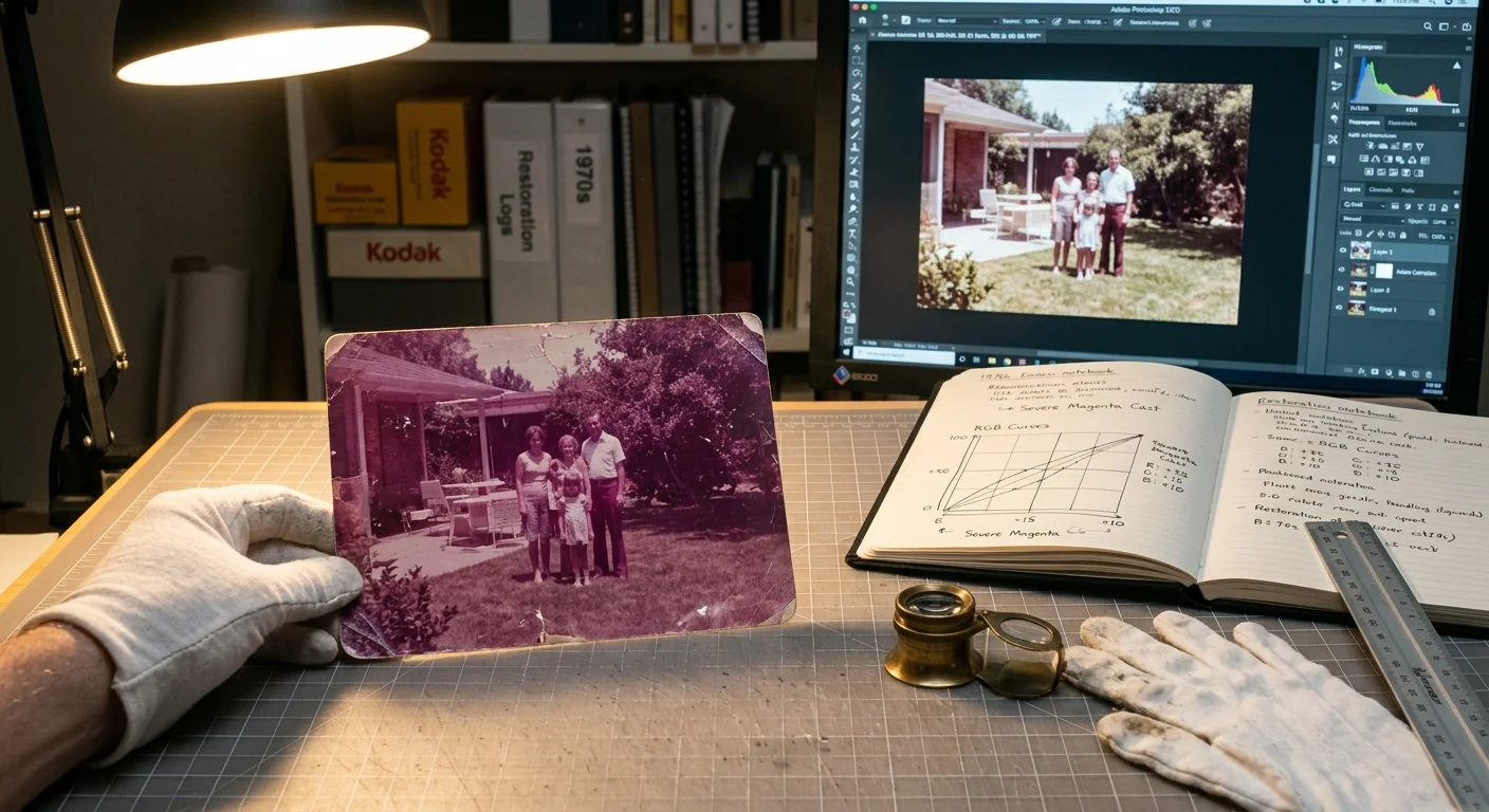
You can salvage family portraits hidden beneath decades of chemical decay by manually rebuilding lost cyan channels. Early 1970s Kodacolor prints fade into severe magenta sheets because cyan coupler dyes decompose first in dark storage.
Standard automated color-balance buttons fail on these prints because they assume balanced dye degradation, leaving faces looking muddy and plastic. You will recover authentic skin tones by plotting precise curve offsets based on surviving shadow density.
This guide details the mathematical Curves formula required to balance cyan dye loss prints without flattening shadow detail or blowing highlight contrast.
The Chemistry Behind 1970s Kodacolor Cyan Dye Loss
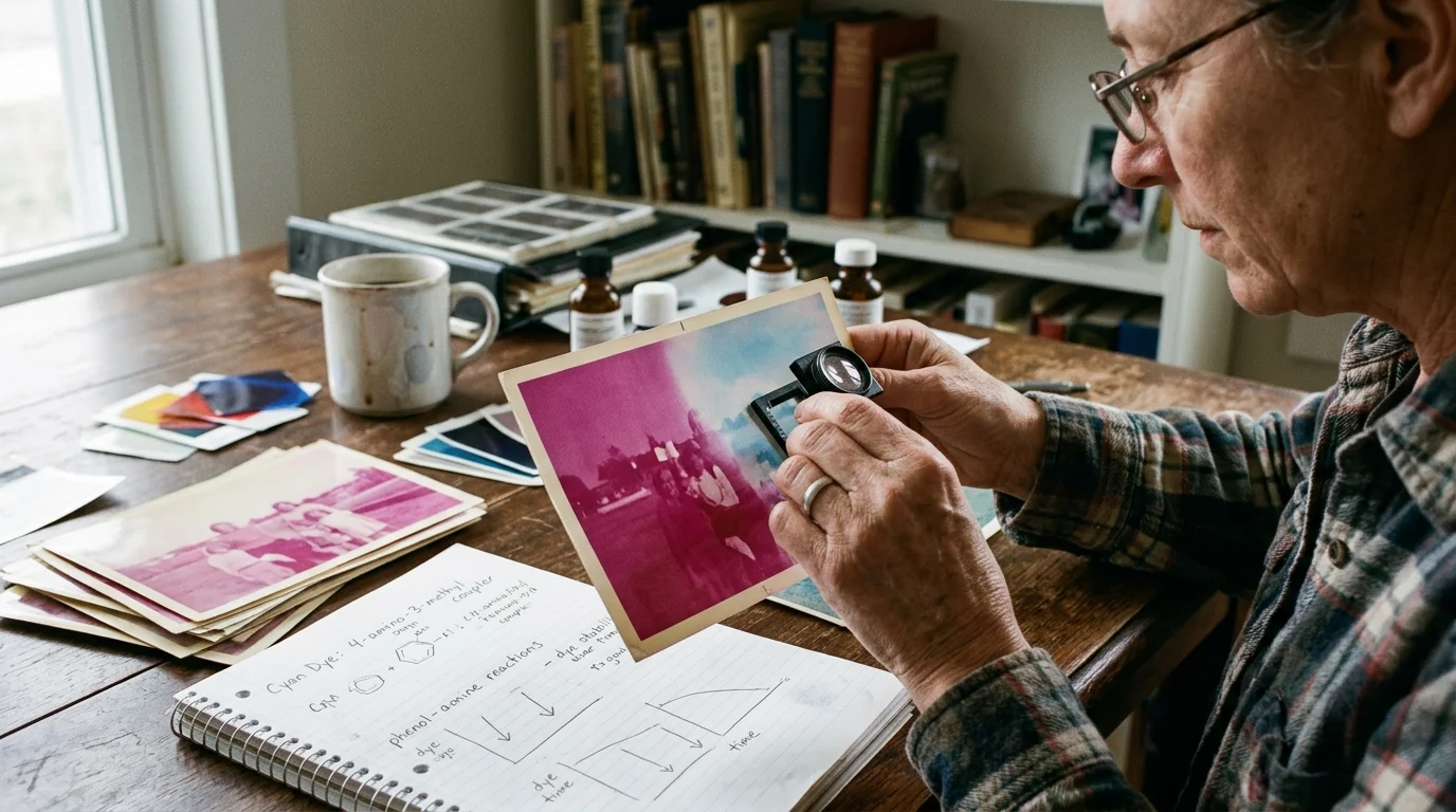
Chromogenic color prints rely on three distinct gelatin emulsion layers sensitized to blue, green, and red light. During chemical processing, oxidized developer reacts with organic dye couplers to generate yellow, magenta, and cyan image dyes.
Prints produced between 1970 and 1977, particularly on Kodak Ektacolor 37 RC paper, contain phenolic cyan couplers. These specific molecules demonstrate poor dark stability when stored at ambient room temperatures.
Research published by the Image Permanence Institute confirms that thermal degradation destroys cyan coupler bonds independently of ambient light exposure. Heat and relative humidity accelerate this breakdown over decades of dark album storage.
While the cyan dye coupler cleaves into colorless chemical byproducts, the pyrazolone magenta dye couplers remain chemically stable. This unequal preservation rate leaves behind an overwhelming magenta cast across every tonal zone.
Genealogists inspecting family albums often misattribute this reddish-purple appearance to sunlight exposure. True light-induced fading bleaches magenta dyes first, whereas dark thermal storage selectively obliterates the cyan emulsion layer.
Thermal dark fading destroys cyan dye couplers while leaving magenta dyes intact. This asymmetric chemical loss causes the intense purple shift seen in 1970s family albums.
Why Auto-Balance Buttons Create Muddy, Desaturated Midtones
Most photo editing software packages feature automatic tone and color correction buttons. These tools analyze the scanned image histogram under the assumption of balanced scene reflectance.
Automated algorithms often apply a mathematical model known as the gray world assumption. This model presumes that the average reflectance of all pixels across a natural scene equals a neutral, middle gray.
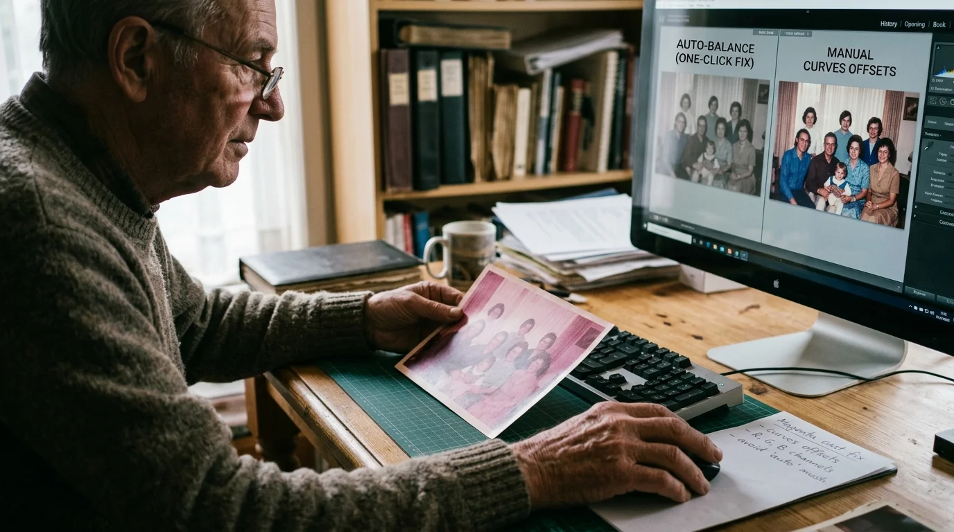
When an algorithm encounters a print suffering from 70% cyan loss, it treats the magenta excess as an exposure imbalance. The software clips the red channel histogram to force the statistical average back toward center.
Clipping the red channel destroys the upper highlight transitions in skin tones, turning subtle facial contours flat and chalky. It creates a lifeless, muddy appearance because it cannot inject synthetic density into depleted tonal channels.
Automated routines also fail to distinguish between base paper yellowing and actual dye loss. Applying automated color fixes invariably produces harsh transitions, posterized shadows, and contaminated highlights.
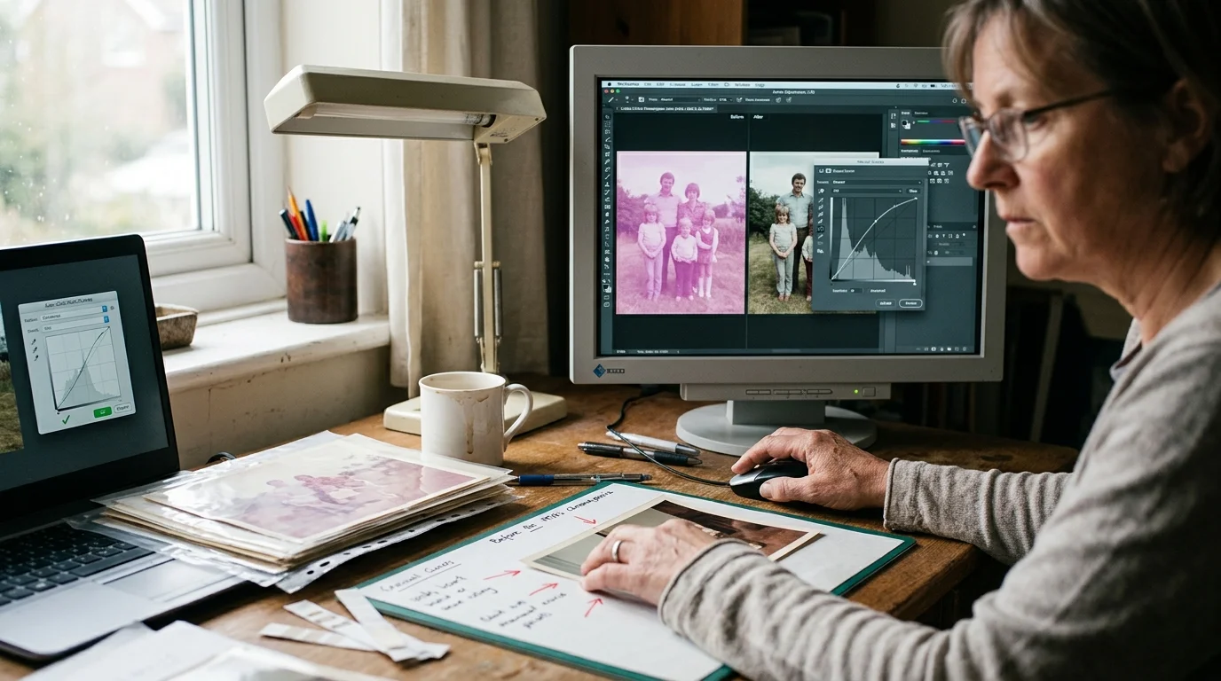
Manual curve offsets give you surgical control over individual tonal anchors. You can restore faded 1970s photos curves by neutralizing color casts without sacrificing your original dynamic range.
Preparing 16-Bit RAW Scans for Precision Curve Adjustments
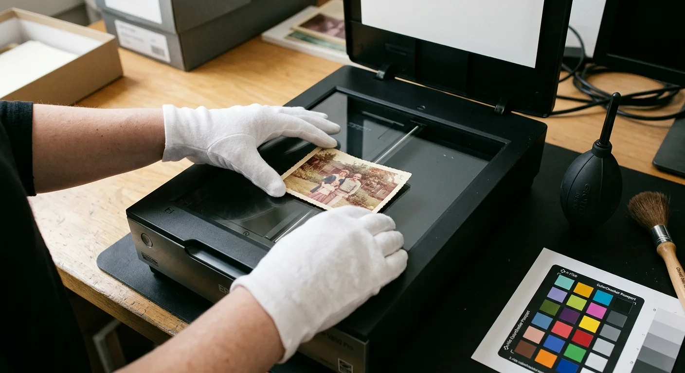
Severe color reconstruction requires substantial histogram stretching across the depleted color channels. You cannot achieve professional restoration quality using standard 8-bit JPEG scans from home flatbed scanners.
An 8-bit file offers only 256 discrete tonal steps per color channel. When you drastically reshape an 8-bit curve, severe comb-like gaps appear in the histogram, resulting in visible banding across smooth backgrounds.
Configure your scanner hardware, such as an Epson Perfection V600, to output 48-bit color, which provides 16 bits per channel. A 16-bit file records 65,536 distinct values per channel, preventing tonal quantization artifacts.
Scan your original prints at a optical resolution of at least 600 pixels per inch (ppi). If you plan to enlarge smaller snapshots, increase optical resolution to 1200 ppi.
Disable all proprietary software optimizations inside your scanning utility prior to acquisition. Turn off automated exposure, unsharp masking, automated color restoration, and infrared dust removal tools like Digital ICE.
Infrared dust suppression relies on infrared absorption, which scatters unpredictably across textured RC photo emulsions. Capture a completely unadjusted, raw linear image file and save it directly as an uncompressed TIFF.
Step-by-Step Formula: Calculating Manual Red and Cyan Curves Offsets
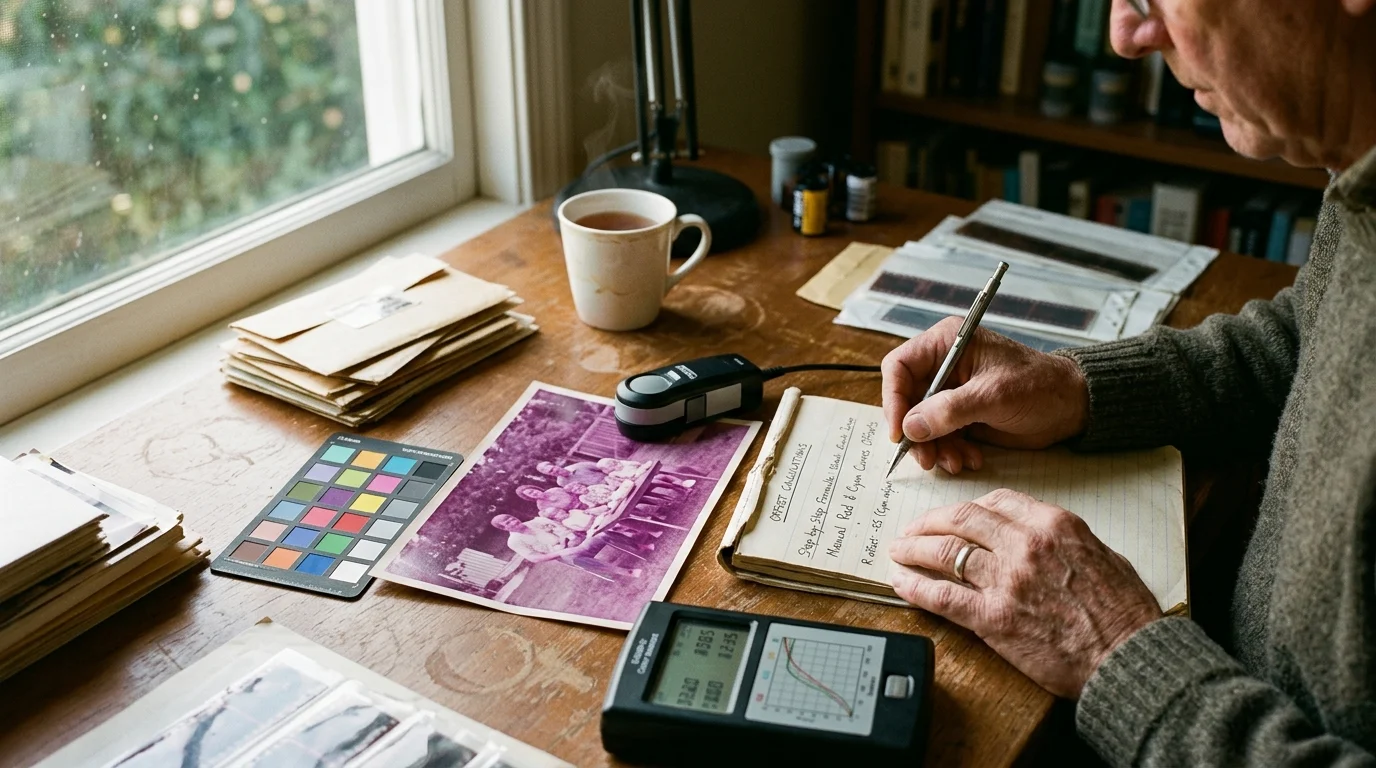
Understanding complementary color geometry is essential when correcting color balance in digital editing software. Digital imaging relies on additive RGB color spaces, where red opposes cyan, green opposes magenta, and blue opposes yellow.
Comprehensive color theory tutorials on Cambridge in Colour illustrate how adjustments along the red curve channel directly manipulate perceived cyan density. Lowering the red curve injects its complementary opposite, cyan, into the image.
Begin by opening your 16-bit TIFF scan in your editing workspace. Create an initial Curves adjustment layer above the background image layer to maintain non-destructive editing workflow practices.
Select the Color Sampler Tool and set the sample size to a 5×5 Average. Point samples read single-pixel noise spikes rather than the true underlying emulsion density.
Locate three distinct reference targets within the composition: a deep shadow, an authentic midtone, and an unclipped highlight. Avoid placing highlight samplers on paper margins, which suffer from distinct chemical yellowing.
Inspect the 8-bit readout equivalents (0 to 255 scale) in your Info panel. In a severely shifted 1970s print, your shadow sampler might display readings like Red 84, Green 26, and Blue 38.
Calculate the primary Red Channel Shadow Offset using the formula: Offset = Red_Shadow – Max(Green_Shadow, Blue_Shadow). In this example, your shadow contains an excess of 46 units of red contamination.
Open the Red channel inside your Curves adjustment dialog box. Place an anchor point at the shadow value and reduce the output value to eliminate the calculated excess.
- Open the RGB Curves panel and switch the active channel from Composite RGB to Red.
- Place an anchor point on the Red curve at the exact input value indicated by your shadow sampler.
- Drag the output value downward until the Red readout matches the highest stable opposing channel reading.
- Switch to the Green channel to neutralize any residual green-magenta imbalance in the midtones.
- Adjust the Blue channel anchor to counter paper base yellowing and restore neutral highlights.
Worked Example: Restoring a Magenta-Shifted 1973 Kodacolor Print
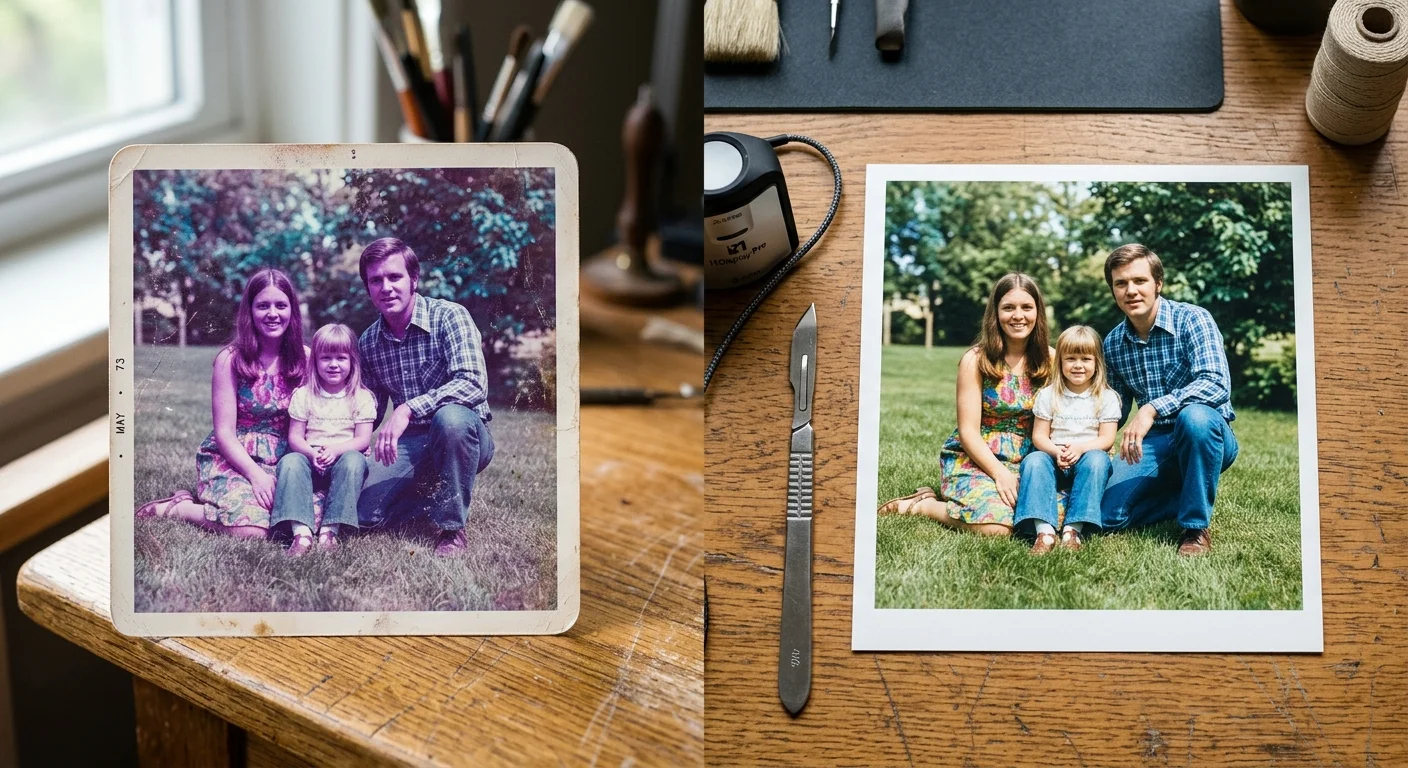
To examine this methodology in practice, consider a 3.5×5-inch Kodacolor II print dated August 1973. The family portrait displays a severe magenta-purple cast across the clothing, skin, and outdoor background.
The uncorrected 16-bit scan reveals strong color imbalance across all measured target zones. The table below lists the initial baseline RGB values recorded using 5×5 sample points.
| Target Zone | Sample Description | Initial Red | Initial Green | Initial Blue | Identified Color Bias |
|---|---|---|---|---|---|
| Shadow (D-max) | Dark Wool Suit Crease | 78 | 24 | 32 | +46 Red (Severe Cyan Deficit) |
| Midtone | Shaded Concrete Porch | 188 | 112 | 136 | +52 Red / -24 Green (Magenta Shift) |
| Highlight (D-min) | Cotton Blouse Fabric | 244 | 192 | 212 | +32 Red / -20 Green (Pink Cast) |
The dark suit crease should register as a neutral shadow. The suit requires balanced RGB values where Red, Green, and Blue match within two tonal steps around 26 to 28.
Select the Red curve and place an anchor point at Input 78. Lower the Output value to 30, which injects cyan directly into the shadows without crushing deepest blacks.
Examine the midtone sampler on the shaded concrete porch, which currently reads Red 188, Green 112, and Blue 136. The green channel displays a massive deficit compared to the surrounding blue values.
Return to the Red curve, place an anchor point at Input 188, and drop the Output value to 128. This step immediately strips the muddy reddish veil from facial features and background elements.
Switch to the Green channel curve to balance cyan dye loss prints without skewing skin tones. Add an anchor point at Input 112 and raise the Output value to 132 to restore missing green spectrum luminance.
Inspect the highlight sampler on the cotton blouse, which now reads Red 212, Green 198, and Blue 212. Switch to the Blue curve, select Input 212, and lower Output to 198 to eliminate cool residual color casts.
The final neutralized readings register at Shadow (28, 27, 28), Midtone (130, 131, 129), and Highlight (198, 198, 197). The manual curves approach successfully restores realistic color relationships without clipping valuable dynamic range.
Manual Curves vs. Automated Tools Comparison
Genealogists frequently rely on automated tools to accelerate large scanning projects. However, automated correction shortcuts degrade the dynamic range of damaged photographic emulsions.
The comparison table below details how four common digital restoration approaches handle severely degraded chromogenic prints. Each method presents measurable trade-offs regarding tone reproduction and channel clipping.
| Restoration Method | Dynamic Range Retention | Shadow Neutrality | Highlight Preservation | Workflow Speed |
|---|---|---|---|---|
| Manual RGB Curve Offsets | 96% – 99% (Unclipped) | Precision Controlled (<2 Delta-E) | Full Texture Intact | 3 – 5 Minutes per Image |
| Photoshop Auto Color | 78% – 84% (Moderate Loss) | Inconsistent (3 – 8 Delta-E) | Frequent Highlight Clipping | Instant (1 Click) |
| Scanner Color Restoration | 65% – 75% (Severe Crushing) | Poor (>10 Delta-E Shift) | Heavy Detail Erasure | Automatic during Scan |
| Generative AI Colorizers | Variable (Alters Pixel Data) | Unpredictable Synthetic Values | Hallucinated Contrast | 30 – 60 Seconds per Image |
Automated scanner firmware adjustments clip both highlight and shadow thresholds to artificially heighten contrast. This destructive clipping permanently discards subtle grain structure and irreplaceable family facial details.
Generative AI restoration tools introduce synthetic color assumptions based on general machine training sets. They invent pigments rather than recovering original coupler dye traces residing inside your photographic emulsion.
Manual curve offsets remain the superior technical method for archival genealogy projects. They respect surviving photographic data while using empirical math to neutralize dye loss.
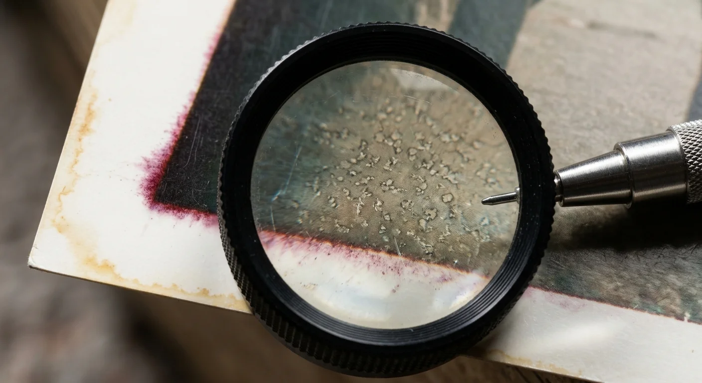
Neutralizing Border Stain and Balancing Uneven Dye Drift
Chromogenic prints rarely degrade at an entirely uniform rate across their entire surface area. Atmospheric gases, acidic album adhesives, and uneven air exposure produce severe edge staining along outer borders.
Inspect the outer margins of your print scan prior to finalizing your color corrections. Edge staining creates a secondary color cast that clashes with corrections applied to the image center.
Never place your white balance or highlight curve anchors on the white paper border of a 1970s print. Optical brightening agents inside resin-coated papers break down into yellow-brown compounds over time.
Calibrating curves against decayed paper borders injects an aggressive blue-cyan cast across authentic scene highlights. Always establish highlight neutral points on interior physical objects like clouds, painted timber, or textiles.
If border stains bleed noticeably into the composition, isolate the affected perimeter using a non-destructive layer mask. Apply a separate, gentle Curves adjustment layer restricted entirely to the perimeter zone.
Lower the global contrast of your peripheral mask to ensure invisible blend transitions between the edges and the center. This layered approach prevents local perimeter staining from distorting your primary image adjustments.
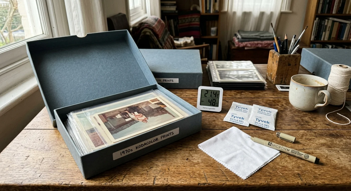
Preserving Original Prints Against Further Dark Fading
Digital restoration salvages the visual information trapped inside degraded emulsions, but physical preservation prevents complete physical loss. You must stabilize your original prints immediately after finishing your digital scanning workflow.
Guidelines established by the Library of Congress Preservation Directorate emphasize rigorous climate control for vulnerable color prints. Thermal dye degradation slows dramatically when environmental temperatures drop.
Store 1970s chromogenic prints at temperatures below 65 degrees Fahrenheit (18 degrees Celsius). For maximum longevity, maintain relative humidity levels consistently between 30% and 40%.
Remove original photographs from vintage self-adhesive magnetic photo albums immediately. The corrugated cardboard backings and aged rubber-based adhesives release volatile acids that accelerate cyan dye destruction.
House your physical prints in archival enclosures made from unbuffered high-density polyethylene, polyester (Melinex), or acid-free paper. Ensure all storage materials pass the rigorous ISO 18916 Photographic Activity Test (PAT).
Store your archival storage boxes upright on metal shelving away from outer exterior walls, basements, and uninsulated attics. Consistent environmental stability ensures your physical family prints survive for subsequent generations to enjoy.
Frequently Asked Questions
Why did 1970s color prints turn magenta while 1950s prints turned yellow?
Dye coupling chemistry changed significantly across photographic eras. Early Kodachrome and vintage dye-transfer prints lost magenta dye first under light exposure, leaving yellow dye dominant.
In contrast, 1970s chromogenic prints suffered from thermally unstable phenolic cyan couplers that degrade rapidly in dark storage, leaving stable magenta couplers intact.
Can I restore faded 1970s photos curves using free software like GIMP?
Yes, you can apply identical mathematical curve offsets inside open-source applications like GIMP. Open the Colors menu, select Curves, and switch between the Red, Green, and Blue channels.
Use GIMP’s Sample Points dialog to monitor real-time RGB values as you manually adjust channel anchor points.
How do I balance cyan dye loss prints when there is no pure white or black in the photo?
Locate objects with known neutral characteristics, such as asphalt roads, gray concrete, overcast clouds, or neutral brown soil. Skin tones also serve as reliable references once you understand standard portrait color ratios.
In standard portraiture, the red channel value in Caucasian, Asian, and African skin consistently exceeds the green value, while green moderately exceeds blue.
Does correcting the magenta cast degrade image quality?
Manual adjustments performed on 8-bit files can cause visible posterization and color banding due to limited tonal data. However, applying manual curve adjustments to 16-bit scans preserves smooth gradients and photographic fidelity.
Disclaimer: This article is for informational purposes only. When handling valuable or irreplaceable photographs, consider consulting a professional conservator. Always test preservation methods on non-valuable items first.